Papers

Most of this research is mathematics where a computer does part of the work (a large search, or a certificate in exact arithmetic). Where I could, I had the Lean proof assistant check the whole proof. If Lean’s kernel accepts a proof that uses only the standard axioms, you only have to trust the kernel and the big-number library that the kernel calls. The kernel is a small checker that anyone can run. You still have to check that the formal statement says what the paper claims.

None of these papers is refereed yet, except the operon paper from my undergraduate project. Where something was checked by machine, the paper’s page says what was checked and under which assumptions. If you find a mistake, please tell me.

Can planets spin as one in only finitely many ways?

Some arrangements of a few bodies in a plane can spin under gravity while the distances between them stay the same. These are central configurations. Euler and Lagrange found the ones for three bodies in the 18th century. The Lagrange points (the James Webb telescope orbits one) come out of those configurations. The next question goes back to Chazy and Wintner. Smale put it on his 1998 list of problems for the next century: for any choice of masses, are there only finitely many central configurations, counting rotated and rescaled copies as one? Hampton and Moeckel answered it for four bodies in 2006. Albouy and Kaloshin answered it for five bodies in 2012, except for masses in a thin exceptional set.

I settled the masses in that exceptional set, so for five bodies in the plane the answer is yes, whatever the masses (the five-body paper). At three special mass ratios the main argument falls short, and I counted the configurations by computer instead. A second paper redoes those cases from the complex solutions of the equations, without the count. A proof of the theorem, including the computations, is checked in Lean from start to finish.

Albouy and Kaloshin’s approach still works for six bodies with generic masses (the six-body paper), but the six-body case for all masses is open. For four bodies, two of the questions left were how many central configurations there are and whether a strictly convex one is unique once you fix the order of the bodies around it. I showed that for almost all masses the number is even and between 32 and 50 (the four-body count paper). I also showed that the strictly convex configuration is unique (the convex paper), and the proof is checked in Lean as well.
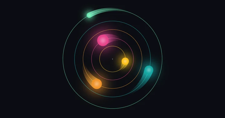
Five glowing coloured discs of different sizes on a dark background, each on its own circle around a common centre, with short fading trails showing them turning counter-clockwise together.

How few multiplications does a 3×3 matrix product need?

Strassen showed in 1969 that two 2×2 matrices can be multiplied with seven multiplications instead of eight. Applied to blocks, over and over, Strassen’s method brings an n×n product down from n³ multiplications to about n2.81. For 3×3 the best known method that works on blocks uses 23 multiplications. Laderman found one in 1976, and nobody had ruled out 22 since.

I ruled out 22 over bits, where 1 + 1 = 0, with a computer search whose result is checked by Lean (the 3×3 paper). Ruling out 22 over bits also rules out 22 for every method with integer coefficients, since such a method can be read mod 2. With arbitrary real coefficients, whether 22 multiplications suffice is still open, and the real-coefficient case is the one I’d most like to see settled.

For 4×4 over bits, a machine-learning search reported in Nature in 2022 found a method with 47 multiplications, and the best lower bound was Bläser’s 34 from 2003. I raised it to 35 (the 4×4 paper). I also took apart five essentially different 47s, every public one that I know of plus a new one, and showed that no group of up to 18 of their multiplications can be replaced by fewer (the rank-47 paper). So a 46, if there is one, shares at most 28 multiplications with any of the five 47s, even allowing for the usual symmetries.

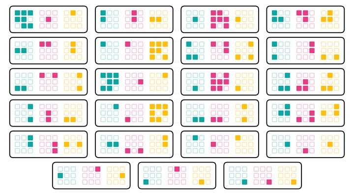
Twenty-three white cards, each with three 3-by-3 grids of small squares in teal, magenta and yellow; the filled squares on each card show the matrix entries used by one product of Laderman's 23-multiplication algorithm for 3-by-3 matrices.

What do genome benchmarks measure?

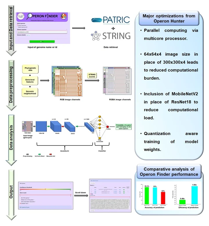
My B.Tech project was a deep-learning model for operons, the runs of neighbouring genes that get switched on together in bacteria and other prokaryotes. It became a web server (Operon Finder) and a 2023 paper in the Journal of Molecular Biology.

A few years later, language models trained on genomes were being pitched as general tools for biology, and operon prediction was one of the tasks they were benchmarked on, so I went back to it. On one such benchmark, scored the benchmark’s own way, a rule that is more than 25 years old beats all 12 protein and genome language models that the benchmark tested. The rule is that neighbouring genes pointing the same way, with a short gap between them, tend to share an operon. In the six benchmarks I looked at closely, much of what they reward can be read off without running any model: where genes sit, and whether a test genome has close relatives in the training data. On 24 of 86 tasks in widely used DNA benchmarks, a simple rule or lookup beats the best published score I could find (the confounds paper). The leaks paper checks 11 recent DNA and RNA benchmarks for copies of training data. The paper comes with seqleak, a tool that automatically finds copy and relatedness leaks.

I also did two smaller audits outside biology. When I reran the Darwin Gödel Machine’s best coding agent on held-out tasks with a newer model, the agent did no better than the version it started from. And before version 1.9, scikit-learn’s GroupKFold could give different folds on different numpy versions and CPUs when group sizes tied.

Figure 1: overview of Operon Finder, with its four stages from top to bottom: input and data retrieval; data preprocessing; data analysis; and output.

How few comparators does a sorting network need?

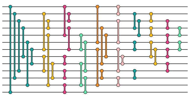
Thirteen numbers need exactly 45 comparators in a sorting network, a fixed list of compare-and-swap operations. Hardware likes such networks because the operations don’t depend on the data. Bose and Nelson asked in 1962 how few comparators you need. Floyd and Knuth answered the question for up to 8 inputs. Codish, Cruz-Filipe, Frank and Schneider-Kamp settled 9 and 10 inputs, and Harder settled 11 and 12. For 13 inputs the best network known, Juillé’s, has 45 comparators, and Dobbelaere’s standard table gave 44 as the lower bound.

But that 44 rested on Van Voorhis’s inequality from 1972, and a 2026 audit found that the inequality’s proof doesn’t hold up. Every lower bound in the table from 13 to 32 inputs rested on that inequality. I first gave each of those 20 bounds a valid proof by counting how many comparators the two largest numbers must meet (the first 13-input paper). Extending the count with a computer search showed that 44 comparators are not enough, so 13 numbers need exactly 45 and every bound from 14 to 32 goes up by one (the second 13-input paper).

For 16 inputs the best network known is Green’s, with 60 comparators. Green found it in 1969, and Knuth includes it in The Art of Computer Programming. I proved that 59 comparators are not enough, so 16 numbers need exactly 60 (the 16-input paper). The proof first shows that 15 numbers need at least 55 comparators. In a 16-input sorting network with 59 comparators, that bound forces the largest number to meet exactly 4 comparators whichever input it enters on, and the same holds for the smallest. The bound of 50 comparators for 14 inputs then narrows the possible paths of the second-largest and second-smallest numbers to a list of candidates, and a computation rules out every one. The same kind of argument shows that 20 numbers need at least 81 comparators. The exact answers for 14 and 15 inputs are still open.

A related problem is selection: networks that only have to pick out the few largest values. For 4 to 18 inputs, I answered Yao’s 1975 question of how few comparators pick out the three largest (the selection-network paper).

Thirteen horizontal black lines crossed by 45 vertical bars with round ends, coloured by layer (ten layers, with six colours repeating), forming the comparator diagram of a 45-comparator sorting network on 13 inputs.

How much noise can the surface code take?

Quantum chips make errors all the time. The standard defence is the surface code, which spreads one reliable qubit over many unreliable ones and keeps correcting their errors. The code works if the hardware’s error rate is below a threshold. Simulations give a rough value for the threshold, but the thresholds that anyone had proved were much lower.

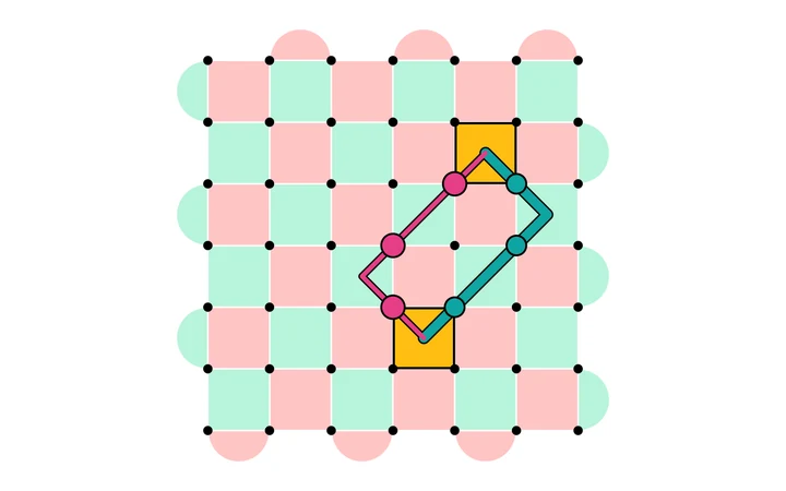
For the standard circuit of the rotated code, decoded by minimum-weight matching, I proved that the code works when every operation, including idling, fails independently with the same probability of up to 0.2%, more than twice what the best earlier guarantee allowed (the circuit-noise paper). In the simpler model where only data qubits flip, each independently of the others, I proved a threshold of at least 4.65% for minimum-weight decoding; no earlier proof reached 4%. On the unrotated code with maximum-likelihood decoding (the best possible repair), a proof and a pre-registered computer experiment certify a threshold of at least 10.3% (the bit-flip paper). Under the conditions stated in that paper, the chance of certifying a false bound this way is at most one in a billion.

A 7-by-7 grid of black dots on a pink and green checkerboard of square tiles, with half-disc tiles along the edges. Lines through three magenta dots and three teal dots form a closed loop that passes through two yellow tiles.

Which entangled states can be distilled?

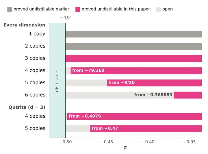
Distillation turns many noisy entangled pairs into fewer clean ones. It has been open since the late 1990s whether every entangled state flagged by the partial-transpose test can be distilled. The question comes down to one family, the Werner states. The two-copy case was settled in July 2026 by four groups independently. I showed that three copies do no better than one (the Werner paper) and proved the underlying inequality for any number of copies on one family of test cases (the Werner paper’s companion).

Christandl’s PPT² conjecture says that two quantum channels of a certain kind (PPT) always destroy entanglement when applied one after the other. I showed that it holds for spin-factor maps in dimension four. The range criterion is the test that certified the counterexample announced in 2026, which has ten-dimensional input and output systems. I also showed that the criterion can’t certify a counterexample when every system has dimension five or less.

A horizontal bar chart on white. Eight bars start at a vertical line marked −1/2, with a pale teal band, labelled distillable, to its left. Under the heading Every dimension, the bars for 1 and 2 copies are grey and the bar for 3 copies is magenta; the bars for 4, 5 and 6 copies begin with light gaps of growing length and turn magenta from −79/160, −9/20 and −0.368683. Under Qutrits (d = 3), the 4-copy bar has a very short light gap before −0.4979, and the 5-copy bar is light until −0.47, then magenta. The axis below is labelled α, from −0.50 to −0.35.

Confinement and percolation on lattices

Quarks are never seen alone. In 1977 Polyakov proposed a mechanism for quark confinement in a simpler model, three-dimensional U(1) lattice gauge theory: the field between two charges gets squeezed into a tube, so pulling them apart costs energy in proportion to the distance. For the standard version of the model, with the Wilson action, confinement had been proved only at strong coupling. I proved it at every coupling by comparing the standard version with the model’s Villain version, for which Göpfert and Mack had proved confinement in 1982 (the area-law paper). The proof runs past a hundred pages, longer than I trust myself to get right, so a companion paper checks all of it in Lean.

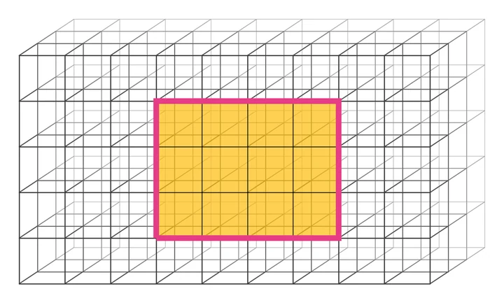
In 1991 Aizenman and Grimmett gave an argument for when locally adding open sites lowers the percolation threshold. Balister, Bollobás and Riordan found a gap in the argument and fixed the proof in dimensions two and three. I proved the claim for every dimension from two up and for 14 other lattices (the enhancements paper). The homological percolation paper proves the mod-2 case left out by Duncan and Schweinhart’s recent theorem on random surfaces wrapping around a torus, for part of the family of models that the theorem covers, a part that includes the four-dimensional Ising gauge theory. So in that theory’s ferromagnetic version, as the torus grows, the cost of every nontrivial ’t Hooft twist goes to zero below Wegner’s self-dual coupling and grows without bound above it.

A box of the cubic lattice drawn in oblique projection, with a thick magenta rectangle four links wide and three links high on the box’s front face. The rectangle encloses twelve yellow-shaded unit squares.

How do you check what a computer did?

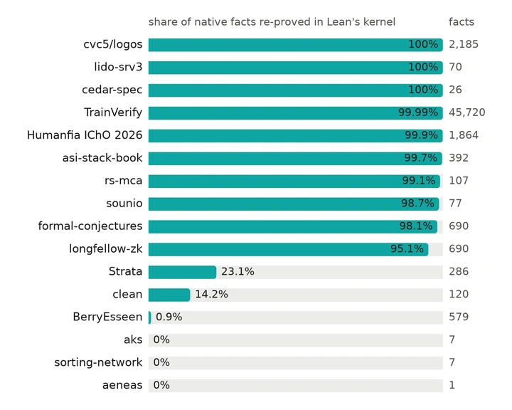
Lean has a shortcut, native_decide, that accepts a fact by running compiled code. The shortcut means trusting the compiler as well as the kernel, and Lean’s main mathematics library doesn’t allow it. I wrote a tool that takes the facts accepted this way by public projects and re-proves them with the kernel alone, without editing the projects (the NativeTrust paper). In 10 of the 16 public projects I studied, the tool re-proves at least 95% of those facts.

Language models can now translate COBOL into Java or Rust, but a translation that passes the tests can still be wrong on inputs nobody tried. So, for the eight standalone batch programs that my COBOL front end can read, taken from AWS’s public CardDemo application, I proved in Lean that their translations behave like the originals on every allowed input (the COBOL paper). The comparison is with the original programs as the paper’s own semantics describes them, and for Java the guarantee holds on every run that finishes.

Horizontal bar chart of 16 packages, sorted by share, each bar on a light grey track from 0 to 100%. cvc5/logos, lido-srv3 and cedar-spec are at 100%, TrainVerify at 99.99%, Humanfia IChO 2026 at 99.9%, asi-stack-book at 99.7%, rs-mca at 99.1%, sounio at 98.7%, formal-conjectures at 98.1% and longfellow-zk at 95.1%; Strata is at 23.1%, clean at 14.2% and BerryEsseen at 0.9%; aks, sorting-network and aeneas are at 0%. A column on the right gives each package's number of native facts, from 45,720 for TrainVerify to 1 for aeneas.

Smaller results

Most of these papers move a known bound on some constant by a little, with a certificate that a computer checks. A few settle a narrow case of a bigger question.